

AI Infrastructure series · Part 9 of 24
The first eight parts of this series were about hardware. This part turns to what runs on it. A large language model (LLM), the technology behind ChatGPT, Claude and Gemini, does one surprisingly simple thing: it predicts the next piece of text, over and over. This post follows that one step all the way through, with real numbers: how text becomes tokens, how a token becomes a row of numbers, how the model scores every possible next token and picks one, how it learns to do that, and which parts of the process decide how much GPU memory, bandwidth and compute you need.
See real tokenizers cut text into tokens, train a tiny BPE vocabulary merge by merge, step through the generation loop with the KV cache growing, and compare temperature and top-p settings for factual answers, creative writing and code.
What does an LLM actually do?
Given some text, an LLM works out how likely every possible next piece of text is. It then picks one piece, adds it to the text, and does the same again with the slightly longer text. A whole answer, a poem or a program is just that one step repeated a few hundred or a few thousand times, until the model picks a special “stop” token or reaches a length limit.
That sounds too simple to produce anything useful. The trick is that predicting well needs a great deal of knowledge. To continue “The capital of France is” the model has to have absorbed geography. To continue a half-written function it has to have absorbed programming. Prediction at this scale behaves like understanding, even though the mechanism underneath is scoring and picking.
What does one prediction look like? A worked example
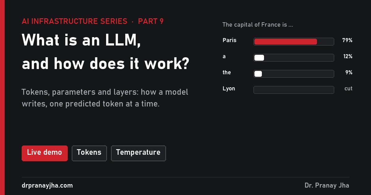
Take the prompt “The capital of France is”. The model does not output a word. It outputs a score, called a logit, for every token in its vocabulary: 128,256 of them for Llama 3.1. Most scores are very low. Here are six of the highest, with made-up but realistic values (illustrative), and how they turn into a choice:
Scores from the model. ” Paris” 8.0, ” a” 5.0, ” the” 4.5, ” located” 4.0, ” Lyon” 3.0, ” home” 2.5. Scores can be any number, positive or negative; only the gaps between them matter.
Make them positive with escore. e8.0 = 2,981, e5.0 = 148.4, e4.5 = 90.0, e4.0 = 54.6, e3.0 = 20.1, e2.5 = 12.2. The total is 3,306.3. A gap of 3 in score becomes a factor of 20 here, which is why the top token pulls so far ahead.
Divide by the total to get probabilities. ” Paris” 2,981 ÷ 3,306.3 = 90.2%, ” a” 4.5%, ” the” 2.7%, ” located” 1.7%, ” Lyon” 0.6%, ” home” 0.4%. They add up to 100%. Steps 2 and 3 together are called softmax.
Draw a random number between 0 and 1. Lay the probabilities end to end: ” Paris” covers 0 to 0.902, ” a” 0.902 to 0.947, and so on, with ” Lyon” covering 0.991 to 0.997. A draw of 0.42 picks ” Paris”. A draw of 0.993 picks ” Lyon”: the model then states, fluently, that the capital of France is Lyon. At these odds that happens in about 1 answer in 165.
Append and repeat. The chosen token joins the text and the whole calculation runs again for the next position, now with ” Paris” in the context.
Every LLM answer is made this way, one draw at a time. The settings that change these odds (temperature, top-k, top-p) come later in this post, and you can watch the draws happen in the demo.
How is text turned into tokens?
Models do not read letters or whole words. Text is first cut into tokens by a tokenizer, and each token is replaced by its number in the model’s vocabulary. Here is a real example, cut by the tokenizer GPT-4o uses (called o200k_base), with each token’s id underneath:
Fourteen words became 16 tokens. Notice three things. The space belongs to the start of the next token, so ” Paris” and “Paris” are different tokens. Punctuation gets its own token. And ” is” has the same id, 382, both times: the model sees the same number wherever the token appears. A rarer word is split into pieces: “Hyperconverged” becomes “Hyper”, “con”, “ver”, “ged”. Numbers are split too: “3.35” becomes “3”, “.”, “35”, which is one reason models are clumsy at arithmetic.
How does a tokenizer decide where to cut? BPE step by step
Most tokenizers are built with byte pair encoding (BPE). Start with every text split into single characters (modern tokenizers start from raw bytes). Count every pair of neighbouring symbols across a large training text. Merge the most common pair into a new symbol, add it to the vocabulary, and count again. Stop when the vocabulary reaches the size you want. The diagram runs this on a tiny corpus, the classic example from the BPE paper for machine translation.
Byte pair encoding on a four-word corpus, computed merge by merge; rows highlight in order. Frequent words end up as one token, rare ones are built from pieces, and nothing is ever unknown because single characters (or bytes) are always in the vocabulary.
Two consequences matter for infrastructure. First, the vocabulary is fixed when the tokenizer is built, before the model is trained, and every model has its own. The same text costs a different number of tokens on different models, so token counts, prices and context limits are only comparable within one tokenizer. Second, the merges reflect whatever text dominated the tokenizer’s training sample. Text that looks like that sample is cut into few, long tokens. Text that does not is cut into many short ones.
| Model | Tokenizer | Vocabulary size | What it means |
|---|---|---|---|
| GPT-2 | byte-level BPE | 50,257 | Mostly English merges; other scripts fall back to bytes |
| Llama 2 | SentencePiece BPE | 32,000 | Small table, more tokens per sentence |
| GPT-4 | cl100k_base | 100,277 | Better coverage of code and European languages |
| Llama 3, 3.1 | tiktoken-style BPE | 128,256 | Four times Llama 2’s table, fewer tokens for the same text |
| GPT-4o | o200k_base | 200,019 | Many more merges for non-Latin scripts |
| Gemma | SentencePiece | 256,000 | Large multilingual table |
Why do other languages use more tokens?
I ran the same sentence, “The capital of France is Paris, and it is known for the Eiffel Tower”, in six languages through three real tokenizers. The counts below are exact for those tokenizers.
| Language | Words | GPT-2 (50K) | GPT-4 (100K) | GPT-4o (200K) | GPT-4o vs English |
|---|---|---|---|---|---|
| English | 14 | 18 | 18 | 16 | 1.0× |
| French | 12 | 18 | 18 | 14 | 0.9× |
| German | 9 | 24 | 17 | 15 | 0.9× |
| Chinese | 19 characters | 42 | 26 | 15 | 0.9× |
| Hindi | 14 | 98 | 68 | 25 | 1.6× |
| Tamil | 8 | 186 | 92 | 29 | 1.8× |
Tokens for the same sentence with GPT-2’s tokenizer, counted with OpenAI’s tiktoken library.
The reason is in how BPE starts. Byte-level tokenizers begin from the bytes of UTF-8 text. An English letter is one byte. A Devanagari or Tamil letter is three. If the tokenizer’s training text had little Hindi, few Hindi merges were learned, and the text falls back to pieces of bytes: the Hindi word for France, six characters and 18 bytes, is 11 tokens for GPT-2. A larger vocabulary trained on more languages fixes most of this, which is why GPT-4o’s tokenizer cuts the Hindi count from 98 to 25. The gap has not gone, and it has real costs: more tokens means a higher bill for the same meaning, a context window that fills sooner, and an answer that takes longer to stream.
Tokens are the unit for everything that follows in this series. Prices are per million tokens (my token cost post works through the maths), speed is tokens per second, the KV cache grows per token, and the context window is measured in tokens. Counting them takes three lines:
import tiktoken
enc = tiktoken.get_encoding("o200k_base")
print(enc.encode("The capital of France is Paris."))
# [976, 9029, 328, 10128, 382, 12650, 13]  -> 7 tokens
What does the model do with a token id?
A token id is just a row number. The first thing inside the model is the embedding table: a matrix with one row per token in the vocabulary and one column per dimension of the model’s internal vector, its hidden size. Looking up row 12,650 gives a list of a few thousand numbers that stand for that token. Nothing is calculated at this point; it is a memory read.
For Llama 3.1 8B the sizes are exact. The vocabulary has 128,256 tokens and the hidden size is 4,096, so the table holds 128,256 × 4,096 = 525,336,576 numbers. At 2 bytes each in 16-bit precision that is about 1.05 GB, just for the lookup table. At the other end of the model sits the output head, a matrix of the same shape, 4,096 × 128,256, that turns the final vector into one score per vocabulary token. Llama 3.1 8B stores it separately (its config sets tie_word_embeddings to false), so the two ends of the model together take another 1.05 billion parameters. This is the hidden cost of a large vocabulary: each extra 1,000 tokens adds 8.2 million parameters to an 8B model.
Llama 3.1 8B shapes. The token id is only a row number; the embedding lookup is a memory read, the layers are where the arithmetic happens, and the output head produces the scores used in the worked example above.
The numbers in each row start random and are adjusted during training until tokens used in similar ways end up with similar vectors. Inside the layers, each token’s vector is updated using the vectors of the tokens before it. That is the attention mechanism, and it is how ” bank” comes to mean something different after “river” than after “loan”. Part 11 follows a vector through one layer in detail.
What are parameters, and where do they live?
Parameters, also called weights, are every number the model learned in training. “8B” means 8 billion of them. They are grouped into matrices, and every matrix has a fixed job. Llama 3.1 8B’s published shapes let you count them exactly:
| Part | Shape | Parameters | Share | 16-bit size |
|---|---|---|---|---|
| Embedding table | 128,256 × 4,096 | 525.3M | 6.5% | 1.05 GB |
| Attention, 32 layers | Q and O 4,096 × 4,096; K and V 4,096 × 1,024 | 1,342.2M | 16.7% | 2.68 GB |
| MLP, 32 layers | three matrices of 4,096 × 14,336 | 5,637.1M | 70.2% | 11.27 GB |
| Norms | vectors of 4,096 | 0.27M | 0.003% | under 1 MB |
| Output head | 4,096 × 128,256 | 525.3M | 6.5% | 1.05 GB |
| Total | 8,030.3M | 100% | 16.06 GB |
K and V are smaller than Q because Llama 3.1 uses grouped-query attention: 32 query heads share 8 key and value heads, each 128 numbers wide. That choice also shrinks the KV cache, as we will see. The 70% in the MLP is typical of dense models, and it is the part that mixture-of-experts models split into many smaller experts (part 12).
Where they live matters more than what they are called. When the model is served, every parameter sits in GPU memory, and every one is read for every token generated, because each new token passes through every layer. That is why 16.06 GB of weights sets both the minimum memory for this model and the time floor for each token (part 7 works out memory for other sizes and precisions).
How does the model write a whole answer?
The generation loop has two phases. In prefill, the whole prompt goes through the model in one pass. While it does, each layer works out a key and a value vector for every prompt token and stores them in GPU memory: the KV cache. Prefill ends with the first set of scores and the first new token. Then decode begins: each step feeds only the newest token through the layers. Its attention needs the keys and values of every earlier token, and reads them from the cache instead of recomputing them. One step produces one token and adds one entry to the cache.
One prefill pass and four decode steps, animated: the stage boxes light up in order and one red token and one cache entry appear per step. KV size per token is Llama 3.1 8B’s 128 KB in 16-bit; token ids and the chosen words are illustrative.
Here is the cache arithmetic for Llama 3.1 8B. Each layer stores a key and a value for each of its 8 KV heads, 128 numbers each, at 2 bytes: 2 × 8 × 128 × 2 = 4,096 bytes per layer. Across 32 layers that is 131,072 bytes, 128 KB per token. A 1,000-token conversation holds about 131 MB of cache. The weights do not change during generation; the cache is the only thing that grows. Without it, step 500 would have to recompute keys and values for all 499 earlier tokens, so total work would grow with the square of the answer length.
The two phases stress different parts of a GPU. Prefill does many calculations per weight read and is limited by compute; it sets the wait for the first token. Decode does about 2 operations per parameter per token, 16 billion for this model, while reading all 16 GB of weights: on an H100 SXM with 3.35 TB/s that is at least 4.8 ms per step, so one user can get at most about 208 tokens per second. Part 13 covers the two phases and part 14 the cache in depth.
How do temperature, top-k and top-p change the pick?
Between the scores and the draw sit a few settings you pass with every request. Temperature divides every score before softmax. Below 1 it widens the gaps, so the top token takes more of the probability. Above 1 it narrows them, so unlikely tokens get picked more often. Temperature 0 is treated as “always take the top token”, called greedy decoding. Top-k keeps only the k highest-scoring tokens and shares the probability among them. Top-p, also called nucleus sampling, keeps the smallest set of top tokens whose probabilities add up to at least p, and drops the rest. Both cut off the long tail of the 128,256 tokens, where the nonsense lives.
Here is what each setting does to the same six scores from the worked example:
| Setting | Paris | a | the | located | Lyon | home |
|---|---|---|---|---|---|---|
| Temperature 0 (greedy) | 100% | 0 | 0 | 0 | 0 | 0 |
| Temperature 0.5 | 99.6% | 0.2% | 0.1% | <0.1% | <0.1% | <0.1% |
| Temperature 1.0 | 90.2% | 4.5% | 2.7% | 1.7% | 0.6% | 0.4% |
| Temperature 1.5 | 73.4% | 9.9% | 7.1% | 5.1% | 2.6% | 1.9% |
| Temperature 2.0 | 59.6% | 13.3% | 10.4% | 8.1% | 4.9% | 3.8% |
| Temp 1.0, top-k 3 | 92.6% | 4.6% | 2.8% | cut | cut | cut |
| Temp 1.0, top-p 0.9 | 100% | cut | cut | cut | cut | cut |
| Temp 1.5, top-p 0.9 | 81.1% | 11.0% | 7.9% | cut | cut | cut |
Two rows deserve a closer look. At temperature 1.0, ” Paris” alone holds 90.2%, which already reaches p = 0.9, so top-p keeps only ” Paris”: a confident distribution is left alone, and a flat one keeps more choices. That adaptiveness is why top-p is more popular than top-k. And at temperature 2.0, ” Lyon” climbs from 0.6% to 4.9%, eight times as likely, without the model’s knowledge changing at all. Settings change how often the wrong answer is drawn, not whether the model knows the right one.
| Use | Typical starting point | Why |
|---|---|---|
| Factual answers, extraction | temperature 0 to 0.3 | One right answer; variety only adds risk |
| Code | temperature 0 to 0.3, top-p 0.95 | A single wrong token can break the program |
| Chat assistant | temperature 0.6 to 1.0, top-p 0.9 to 0.95 | Natural wording that does not repeat itself |
| Creative writing, brainstorming | temperature 0.9 to 1.2, top-p 0.95 | Less likely words are the point |
Common starting values, not rules; model makers often publish their own recommended settings, and these should come first.
In practice the settings travel with each request to a model server. This is the OpenAI-compatible API that vLLM and most other servers expose (part 16):
curl http://localhost:8000/v1/completions -H "Content-Type: application/json" -d '{
  "model": "meta-llama/Llama-3.1-8B-Instruct",
  "prompt": "The capital of France is",
  "max_tokens": 20, "temperature": 0.2, "top_p": 0.9, "logprobs": 5 }'
# "logprobs": 5 returns the top five candidates and their log-probabilities
# for each generated token; "usage" in the reply counts prompt and completion tokens
Why are models confidently wrong?
Look again at the draw. The model produces the most likely continuation given its training, not a checked fact. There is no step where it looks something up or asks itself whether it is sure. Fluency comes from the same process as accuracy, so a wrong token is written in exactly the same confident style as a right one. When a fact was rare in the training text, such as a minor court case, a specific part number or a quote, the right answer may score little higher than several plausible wrong ones, and the model picks one of them. This is what people call hallucination. Lower temperature helps when the right answer is clearly on top; it cannot help when it is not. Grounding the answer in retrieved documents, as RAG systems do, puts the right text into the context so it scores highest. That reduces wrong answers but does not remove them.
What is a context window, and what happens when it fills?
The context window is the most tokens the model can consider in one request: prompt plus answer. Llama 3.1 supports 128K (131,072) tokens. Everything the model knows about your conversation has to fit in it: the system prompt, tool definitions, retrieved documents, the earlier turns, the new question and room for the answer.
Segment sizes are an illustrative mix for a RAG chat app. The KV figure uses Llama 3.1 8B’s published shapes in 16-bit: one full-length request needs about as much memory as the model itself.
The model itself never sees anything outside the window, and it does not choose what to drop: the server or the application decides. A model server such as vLLM refuses a request that cannot fit inside its configured maximum length. Chat applications quietly cut or summarise the oldest turns, which is why a long chat can “forget” something you said at the start. The cost of a long window is mostly memory, not weights: each token of context is 128 KB of KV cache for every concurrent request, and every decode step reads all of it. That is why a server is usually configured with a maximum length far below what the model supports.
How does a model learn?
Training adjusts the parameters so that the scores in the worked example come out right. The model reads a passage, predicts each next token, and the training code measures how much probability it gave to the token that really came next. Back-propagation then nudges every parameter a tiny amount in the direction that would have raised that probability. Repeated over trillions of tokens, the nudges add up to grammar, facts, style and reasoning habits. It happens in stages, and the stages differ in size by orders of magnitude.
Data sizes are the published ranges in the table below; the replies are illustrative. Each stage starts from the previous stage’s weights, so later stages shape behaviour rather than add much knowledge.
| Stage | Data | Published examples | Hardware |
|---|---|---|---|
| Pre-training | Raw text and code, next-token prediction | GPT-3: 300B tokens. Llama 2: 2T tokens. Llama 3: over 15T tokens | Thousands of GPUs for weeks or months; Llama 3.1 405B used up to 16,000 H100s |
| Instruction tuning (SFT) | Prompts with written model answers | InstructGPT: about 13K prompts. Llama 2: 27,540 annotated examples | Tens to hundreds of GPUs, hours to days |
| Preference tuning (RLHF, DPO) | Pairs of answers ranked by people or models | InstructGPT reward model: 33K prompts. Llama 2: over 1 million comparisons | Similar to SFT; RLHF also runs a reward model and generates answers during training |
| Reasoning RL (optional) | Problems whose answers can be checked automatically | Varies; few makers publish sizes | Heavy on inference: the model writes long attempts to be scored |
| Your fine-tuning | Your own examples, often a few thousand | LoRA trains well under 1% of the parameters | One GPU to a few servers (part 19) |
Pre-training is where knowledge comes from, and it is the stage almost nobody repeats. A useful rule from the Chinchilla paper (Hoffmann et al., 2022) is that compute is best spent on about 20 training tokens per parameter. Modern small models go far past that on purpose: Llama 3 8B saw over 15 trillion tokens, nearly 1,900 per parameter, because a small model that is cheap to serve is worth extra training. Training compute is about 6 × parameters × tokens, so for that model: 6 × 8.03 billion × 15 trillion ≈ 7.2 × 10²³ operations, which Meta’s model card puts at 1.46 million H100 GPU hours for Llama 3.1 8B.
What is the difference between base, instruct and reasoning models?
| Kind | Stages applied | Behaviour | Typical use | Infrastructure effect |
|---|---|---|---|---|
| Base | Pre-training only | Continues any text; does not follow instructions reliably | Starting point for your own fine-tuning | Same size and speed as the instruct version |
| Instruct or chat | Plus SFT and preference tuning | Answers questions, follows a chat template, refuses some requests | Assistants, RAG, most applications | Same weights shape; usually what you serve |
| Reasoning | Plus reinforcement learning on checkable problems | Writes a chain of working before the answer | Maths, code, multi-step planning, agents | Many more output tokens per answer: more decode time, more KV cache, higher cost |
On a model hub these usually appear as separate files with the same architecture, such as Llama-3.1-8B and Llama-3.1-8B-Instruct. The memory needed to serve them is identical. A reasoning model can be the same size too; what changes is that it may decode hundreds or thousands of hidden thinking tokens before the visible answer, and every one of them costs a decode step and a KV cache entry.
What does an LLM need from hardware at each stage?
Put the pieces together for one model, Llama 3.1 8B, and the hardware needs line up with the earlier parts of the series:
| Stage | Memory | Bottleneck | Worked number | Read more |
|---|---|---|---|---|
| Pre-training | About 16 bytes per parameter (weights, gradients, optimizer state): 128 GB before activations | Compute and the network between GPUs | 7.2 × 10²³ operations, 1.46M H100 GPU hours | part 15 |
| Full fine-tuning | Same 16 bytes per parameter: more than one 80 GB GPU | Memory | 128 GB, so shard across 2 or more GPUs | part 19 |
| LoRA fine-tuning | 16 GB frozen weights plus a small adapter | Memory | Rank 16 on all 7 matrices: 41.9M parameters, about 84 MB | part 19 |
| Inference, prefill | 16 GB weights plus KV for the prompt | Compute | 2 × 8.03B = 16 GFLOPs per prompt token | part 13 |
| Inference, decode | 16 GB weights plus 128 KB per token per request | Memory bandwidth | 16 GB ÷ 3.35 TB/s = 4.8 ms a step, at most about 208 tokens/s for one user on an H100 | part 4, part 14 |
Serving many users changes the picture again, because one read of the weights can serve a whole batch of requests at once. That is the subject of the serving parts, from part 16 onwards.
What do people get wrong about LLMs?
- “It looks things up.” A model on its own has no database and no internet. Everything it knows is spread across its weights, as of its training cut-off. When a product does search the web or your documents, a separate system fetches text and places it in the context window, and the model reads it there.
- “It remembers me.” Weights do not change when you chat; inference only reads them. Each request starts from nothing except what is in its context. Chat “memory” features work by saving notes and inserting them into later prompts, which costs tokens like any other text.
- “Bigger is always better.” Training data and tuning matter as much as size. The Chinchilla paper’s 70B model beat the 280B Gopher model by training on more than four times the data. A well-trained 8B model that fits one GPU often serves a narrow task as well as a much larger one, at a fraction of the cost.
- “Temperature 0 gives the same answer every time.” It removes the random draw, but tiny floating-point differences from batching on GPUs can still flip a close call between two tokens, and one different token changes everything after it. Expect near-identical, not guaranteed identical.
- “A token is a word.” In English a token averages about three quarters of a word, and in many other languages a word can be several tokens. Size budgets and price estimates in tokens, never in words.
- “A longer context window is free.” The window is a limit, not a cost. The cost is the KV cache for the tokens you actually send, multiplied by the number of users at once.
Short answers to common questions
Does an LLM understand what it writes?
It builds internal representations good enough to predict text across almost any subject, which behaves like understanding for many tasks. It has no separate step that checks facts, so treat its output as a strong draft, not a source.
Why does the same question get different answers?
Because each token is a random draw from a distribution. With temperature above 0, a different early token sends the rest of the answer down a different path.
How many tokens is a page of text?
About 500 words of English is roughly 650 to 700 tokens on a modern tokenizer. The same page in Hindi or Tamil can be one and a half to two times that, and several times more on older tokenizers.
Can I change what a model knows without retraining it?
For facts that change, put them in the prompt with retrieval (RAG). For behaviour, format or a narrow skill, fine-tune with LoRA. Pre-training again is almost never the answer.
- Number of parameters, times bytes per parameter: the memory for weights (part 7).
- Context length and number of users: the size of the KV cache.
- Prompt length: prefill time, which is compute-bound.
- Answer length, including any hidden reasoning tokens: decode time, which is memory-bandwidth-bound.
- Your tokenizer and language: the same text can cost very different token counts.
- Whether you only run the model, or also fine-tune or train it.
Token ids and counts were produced with OpenAI’s tiktoken library (gpt2, cl100k_base and o200k_base encodings). The BPE example follows Sennrich et al. (2016) and was computed merge by merge. Llama 3.1 8B shapes and vocabulary are from its published model config; GPU hours and training tokens are from Meta’s Llama 3 paper and model card. Llama 2 data sizes are from the Llama 2 paper (Touvron et al., 2023), InstructGPT sizes from Ouyang et al. (2022), GPT-3 tokens from Brown et al. (2020), the 20 tokens per parameter rule and the Gopher comparison from Hoffmann et al. (2022). Gemma’s vocabulary is from Google’s Gemma documentation. Logit scores, context mixes, sampling presets and example replies are illustrative; bandwidth figures are ideal ceilings.
About The Author







 DrJha