

AI Infrastructure series · Part 15 of 24
Most of the AI hardware news is about training: thousands of GPUs, months of work, one huge run. Most of the AI infrastructure that companies actually build is for inference: answering questions with a model that is already trained. Both run on the same GPUs, but they use memory, network and time very differently. This part works through each difference with numbers, using Meta’s Llama 3.1 as the example, and explains why a cluster built for training is not automatically a good production platform.
Four tabs. Build the training memory of Llama 3.1 8B, 70B or 405B per GPU with activations, checkpointing and ZeRO sharding. Work out the GPU hours of a training run. Watch serving traffic overtake the training compute. Then share one cluster between training and inference over a day.
What is the difference between training and inference?
Training is how a model learns: it predicts the next token at every position of trillions of tokens, measures how wrong it was, and nudges every weight a little. Inference uses the finished model: the weights are frozen, a prompt goes in, tokens come out. Training changes the weights; inference only reads them.
That one difference drives everything else in this post. To change a weight you need to know how it affected the result, so training has to keep extra numbers for every weight and every intermediate value. To only read the weights, inference needs the weights and the KV cache (part 14) and nothing else. The diagram runs one training step next to one inference request, with a memory bar for each drawn to the same scale.
Both memory bars use one scale: the black W block is 2 bytes per parameter of 16-bit weights. Training adds gradients, optimizer state and activations that grow in the forward pass and are freed in the backward pass. Serving adds a KV cache per request; the rest of the GPU holds other users’ requests.
Where does each job sit in a model’s life?
Pre-training and post-training are usually done by the model maker. Most companies start from an open model, fine-tune it on their own data if needed, and serve it. For most readers the platform to design is for fine-tuning and serving, not pre-training.
GPU counts and durations are typical ranges, not fixed rules. Fine-tuning with LoRA (part 19) can run on a single GPU; serving a very large model can take a whole rack per copy.
What happens in one training step, step by step?
A training run is one loop repeated until the token budget is used. With batches of up to 16 million tokens, Llama 3.1 405B’s 15.6 trillion tokens is in the order of a million steps. Every step does four things on every GPU:
Forward pass. Each GPU runs its share of the batch (say 16 sequences of 8,192 tokens) through every layer, as inference would, but keeps every layer’s intermediate results (the activations) for the backward pass. About 2 × parameters operations per token.
Loss. How much probability the model gave to the token that really came next, averaged over the batch. One number, logged every step.
Backward pass. Working back from the loss through the layers, using the stored activations, the GPU calculates a gradient for every weight: how the loss would change if that weight moved. About twice the forward work, 4 × parameters per token, which is where 6 × parameters × tokens comes from.
All-reduce and update. Each GPU saw different data, so the GPUs average their gradients over the network (an all-reduce). Adam then updates every weight. The next step cannot start until every GPU is done, so all wait for the slowest.
An inference request is only step 1, with no loss, no backward pass and nothing kept except the KV cache. Its forward pass splits into prefill, which handles the whole prompt at once, and decode, one token per pass (part 13). Prefill keeps the Tensor Cores busy like training. Decode reads every weight from memory to produce one token per user, so it is limited by memory bandwidth (part 4), not compute.
Where does every byte of training memory go?
To serve a model in 16-bit you need 2 bytes per parameter for the weights, plus the KV cache. To train it with the usual mixed-precision Adam setup, every parameter carries much more. Here is the breakdown for one parameter, from the ZeRO paper:
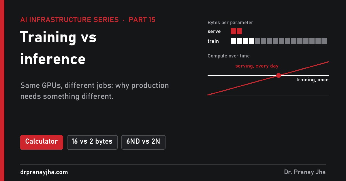
Why so many copies? The passes run in 16-bit because it is fast, but a single update is often too small to register in 16-bit, so the optimizer applies it to a 32-bit master copy. Adam also keeps a running average of each weight’s gradients and of their squares, which sets the size of each weight’s step. Every parameter costs 16 bytes, 8 times what serving needs.
| Model | Weights to serve (16-bit) | Training state (16 bytes/param) | 80 GB GPUs just to hold the state |
|---|---|---|---|
| Llama 3.1 8B | 16 GB | 128 GB | 2 |
| Llama 3.1 70B | 140 GB | 1.12 TB | 16 |
| Llama 3.1 405B | 810 GB | 6.5 TB | 90 |
Why do activations grow with batch and sequence length?
The 16 bytes are fixed per parameter. Activations are not: they are the values flowing through the model, so they scale with how much data is in flight. Korthikanti et al. (NVIDIA, 2022) worked out that a standard transformer layer stores about 34 × s × b × h bytes of activations in 16-bit, where s is the sequence length, b the number of sequences on the GPU (the micro-batch) and h the hidden size, plus a term for the attention scores that modern attention kernels such as FlashAttention do not keep. Multiply by the number of layers and you have the activation memory.
For Llama 3.1 8B (hidden size 4,096, 32 layers) with one sequence of 8,192 tokens: 34 × 8,192 × 1 × 4,096 = 1.14 GB per layer, × 32 layers = 36.5 GB. That is more than twice the 16 GB of weights, for a single sequence. Double the sequence and it doubles; put 4 sequences on the GPU and it is four times as much.
These are rough, illustrative estimates (Llama’s MLP is larger than the textbook layer), but the shape is right.
Activation checkpointing is the standard fix. Instead of keeping every intermediate value, the GPU keeps only each layer’s input (2 × s × b × h bytes) and recomputes the rest of that layer during the backward pass. For the 8,192-token example that is 2.15 GB of saved inputs plus about 1.14 GB for the one layer being recomputed: about 3.3 GB instead of 36.5 GB. The cost is an extra forward pass, so the step needs roughly 8 × parameters × tokens operations instead of 6, about a third more compute. Selective checkpointing, which recomputes only the cheapest parts, keeps most of the memory saving for a fraction of that cost: the same paper reports 5 times less activation memory while cutting the recomputation overhead by over 90%.
How does sharding spread the training state across GPUs?
With plain data parallelism (PyTorch DDP), every GPU holds a full copy of the weights, gradients and optimizer state and works on different data. For the 8B model that is 128.5 GB per GPU, which does not fit on an 80 GB GPU no matter how many GPUs you add. The ZeRO paper (Rajbhandari et al., Microsoft) pointed out that this is wasteful: every GPU stores identical optimizer state. Its three stages split that state across the data-parallel GPUs, one more piece at a time. PyTorch’s FSDP implements the same ideas.
Drawn for four GPUs. A sharded block means each GPU keeps only its quarter and the others keep the rest. Memory figures use the ZeRO paper’s formulas for Llama 3.1 8B (8.03B parameters) and exclude activations, which come on top.
Stages 1 and 2 are almost free: each GPU only needs its own slice of optimizer state, and gradients can be reduced straight to the GPU that owns them, so traffic matches plain data parallelism. Stage 3 also splits the weights, so the GPUs gather each layer’s weights before using it and drop them afterwards, about 1.5 times the traffic. In PyTorch FSDP the choices are NO_SHARD (DDP), SHARD_GRAD_OP (like stage 2), FULL_SHARD (stage 3) and HYBRID_SHARD, which shards inside a node and replicates across nodes to keep the gathers on NVLink.
| Stage | What is split | 8B on 8 GPUs, per GPU | 70B on 64 GPUs, per GPU |
|---|---|---|---|
| DDP | Nothing | 128.5 GB | 1,130 GB |
| ZeRO-1 | Optimizer state | 44.2 GB | 296 GB |
| ZeRO-2 | Optimizer state and gradients | 30.1 GB | 157 GB |
| ZeRO-3 / FSDP full shard | Everything, gathered layer by layer | 16.1 GB | 17.7 GB |
Sharding divides the 16 bytes by the number of GPUs. It does not divide the activations, because each GPU still processes its own sequences. Large runs therefore combine sharding with tensor parallelism and pipeline parallelism (part 5), which split each layer and the stack of layers across GPUs and do reduce activations per GPU. Meta trained Llama 3.1 405B with tensor parallelism of 8 inside each server, 16 pipeline stages, and FSDP-style sharding across the data-parallel groups.
How much compute did Llama 3.1 405B need?
Training costs about 6 × parameters × training tokens operations, and the GPU hours follow from how fast the GPUs really run. Here is the calculation step by step, so you can repeat it for any model.
Operations. 6 × 405 × 109 parameters × 15.6 × 10¹² tokens = 3.79 × 1025. Meta reports 3.8 × 1025, so the rule of thumb holds.
Real speed per GPU. An H100 SXM peaks at 989 TFLOPS dense in BF16. Nothing runs at peak, so multiply by the model FLOPs utilisation (MFU), the share of peak that goes into useful model maths. Meta measured 38% to 43%. At 40%: 989 × 0.40 = 396 TFLOPS per GPU.
GPU seconds. 3.79 × 1025 ÷ 3.96 × 1014 = 9.58 × 10¹⁰ GPU seconds.
GPU hours. ÷ 3,600 = 26.6 million H100 hours at 40% MFU (24.8 million at 43%, 28.0 million at 38%).
Compare with the real run. Meta reports 30.84 million GPU hours, about 16% more than step 4. The gap is time when the GPUs were not doing useful maths: restarts after failures, the long-context phase at lower MFU, checkpoint writes and evaluation. On 16,384 GPUs, 30.84 million hours is about 1,880 hours, roughly 78 days of wall-clock time.
MFU depends on how the job is split. Meta published three of its configurations, and the trend is general: more GPUs and longer sequences mean more time spent communicating and less doing maths.
| GPUs | Parallelism (TP, CP, PP, DP) | Sequence length | TFLOPS per GPU | MFU |
|---|---|---|---|---|
| 8,192 | 8, 1, 16, 64 | 8,192 | 430 | 43% |
| 16,384 | 8, 1, 16, 128 | 8,192 | 400 | 41% |
| 16,384 | 8, 16, 16, 8 | 131,072 | 380 | 38% |
Meta’s model card lists 1.46 million GPU hours for 8B and 7.0 million for 70B, on the same 15 trillion-plus tokens: cost scales with parameters × tokens.
Why does inference end up using more compute than training?
The training bill is paid once. Inference is paid on every token, for as long as the model is in use. A served token costs about 2 × parameters operations; a training token cost 6 × parameters. So serving has used as much compute as training once it has processed about three times the training tokens. Model size cancels out: the crossing point depends only on how many tokens the model was trained on and how much it is used.
For Llama 3.1 that is 3 × 15.6 trillion = 46.8 trillion tokens. Each served token on the 405B model costs 2 × 405 × 109 = 8.1 × 10¹¹ operations. A service handling 100 billion tokens a day (illustrative) adds 8.1 × 10²² operations a day and matches the training compute after 46.8 trillion ÷ 100 billion = 468 days, about 15 months.
Operations only, for Llama 3.1 405B. Traffic levels are illustrative. A model used at 1 trillion tokens a day passes its training compute in about 47 days; at 10 billion it takes over a decade.
In GPU hours the crossing comes even sooner, because inference runs at a much lower share of peak. Decode is limited by memory bandwidth, so serving GPUs often reach only a small fraction of their peak operations. Suppose the 405B service runs at 10% MFU (illustrative): 8.1 × 10²² operations a day ÷ (989 × 1012 × 0.10) = 8.2 × 10⁸ GPU seconds, about 227,000 H100 hours a day, or 9,500 H100s busy around the clock. At that rate the 30.84 million training hours are matched in about 136 days, not 468. This is why serving efficiency (batching, quantization, caching, covered in parts 17 and 18) is where most of the money is.
How do network traffic and failures differ?
Why does training need such a fast network?
At the end of every training step, every GPU must share its gradients with every other GPU in its data-parallel group before any of them can update. With the ring all-reduce used by NCCL, each GPU sends and receives about 2 × (N − 1) ÷ N times the gradient size. For the 8B model, 16 GB of 16-bit gradients means roughly 32 GB in and 32 GB out per GPU, every step. On a 400 Gb/s link (50 GB/s) that is about 0.64 seconds (illustrative), which frameworks hide by overlapping it with the backward pass, layer by layer. If the network is slower than the backward pass, the GPUs sit idle, and because all GPUs move in lock step, one slow link slows all of them.
Gradient sizes are for Llama 3.1 8B in 16-bit; the per-step figure is the standard ring all-reduce volume. Inside one inference replica that spans several GPUs, tensor parallelism does exchange activations at every layer, but that traffic stays on NVLink inside the server.
Inference traffic is the opposite: a 2,000-token prompt is about 8 KB of text and the answer a few KB. Replicas are independent, so the network between servers carries requests, responses and model downloads. The fast traffic is inside a replica: a 70B model split over 4 or 8 GPUs runs two all-reduces per layer per token, so serving servers need NVLink but rarely a rail-optimised fabric between them (part 8).
What happens when a GPU fails?
A training run is one job spread over thousands of GPUs. If one GPU fails, the whole job stops, because no step can finish without it. Meta’s paper reports 466 job interruptions in a 54-day period, 419 of them unexpected, with about 78% caused by confirmed or suspected hardware problems and faulty GPUs the largest single cause. Recovery means finding the bad node, replacing it and reloading the last checkpoint. Everything computed since that checkpoint is lost.
Timings are illustrative. Training trades checkpoint frequency against lost work; inference trades spare replicas against the chance of overload during a failure.
Worked example (illustrative): 419 unexpected interruptions in 54 days is about 7.8 a day on a 16,384-GPU job. If checkpoints are taken every 30 minutes, an average failure loses 15 minutes of work; add 10 minutes to restart and that is 25 minutes × 16,384 GPUs = 6,800 GPU hours per failure, or about 53,000 a day out of the 393,000 GPU hours the cluster has each day: 13.5% wasted. Checkpointing every 10 minutes cuts that to about 8%. Meta reported over 90% effective training time, which needs both frequent checkpoints and fast restarts. Each checkpoint is large: the full training state of the 405B model is 16 bytes × 405 billion = 6.5 TB, written in bursts that Meta notes can saturate the storage fabric. That is why training clusters need a fast parallel file system and inference clusters mostly do not.
An inference service cannot stop for a restart. It runs independent replicas behind a load balancer with enough spare capacity that the survivors carry a failed copy’s users while a replacement loads. Requests that were mid-answer must be retried, but nobody waits for a cluster-wide restart.
Which GPUs suit which job?
Training wants the most compute, the fastest links between GPUs and enough memory for the training state. Inference wants memory capacity and bandwidth for weights and KV cache, and is often happy without NVLink if the model fits on one GPU. That opens up cheaper cards for serving that would be poor training choices.
| GPU | Memory and bandwidth | Training | Inference |
|---|---|---|---|
| H100 SXM | 80 GB, 3.35 TB/s, NVLink 900 GB/s | Standard choice for large runs | Strong; 70B needs 2 or more in 16-bit |
| H200 | 141 GB, 4.8 TB/s | Same compute as H100, more room for state and activations | Very good: more KV cache, faster decode |
| B200 | 192 GB, 8 TB/s | Frontier training | Largest models, highest throughput per GPU |
| L40S | 48 GB GDDR6, 864 GB/s, no NVLink | Small models and LoRA only; PCIe limits multi-GPU | Good for models that fit in 48 GB, such as 8B or a quantized 70B on two cards with care |
| RTX 4090 | 24 GB, 1,008 GB/s | Experiments, QLoRA on small models | Development and small models; not a data-centre card |
The bottleneck moves between jobs. In training the 989 TFLOPS is the limit; in decode the 3.35 TB/s is, so an H200 with 43% more bandwidth decodes faster on the same chip compute (part 7 sizes models to GPUs).
What changes in operations?
A training run is operated like a long batch job. A production inference service is operated like any customer-facing service, with very large processes on scarce hardware.
| Area | Training | Inference |
|---|---|---|
| What you promise | Finish within budget and time | SLOs: time to first token, time per output token, error rate |
| Scaling | Fixed GPU count for the whole run | Autoscale replicas on queue length or KV cache use; a replica takes minutes to load the model |
| Changes | New run, new checkpoint | Rolling or canary rollouts of new models and engine versions, with rollback |
| Failure | Restart from checkpoint | Spare replicas, health checks, retries |
| Security | A fixed, approved dataset | Customer data in every prompt: authentication, rate limits, tenant separation, logging rules |
| Main metric | Tokens per second, MFU, loss | Latency percentiles and cost per million tokens |
How does it look in practice?
A training job is launched once per node and the processes find each other over the network. A typical two-node PyTorch launch, and the kind of line a training loop logs every step (values illustrative):
# run on each of 2 nodes, 8 GPUs each
torchrun --nnodes=2 --nproc_per_node=8 \
  --rdzv_backend=c10d --rdzv_endpoint=node0:29500 train.py

# what the log shows, every step
step 41200 | loss 1.92 | 395 TFLOPS/GPU | MFU 40% | 2.1 s/step
A sudden drop in TFLOPS usually means one slow GPU or link; a loss spike can mean bad data. A serving engine is a long-running server behind a load balancer, monitored like an API:
# one replica of an 8B model, OpenAI-compatible API on port 8000
vllm serve meta-llama/Llama-3.1-8B-Instruct --gpu-memory-utilization 0.9

# what you alert on (Prometheus metrics from the engine)
vllm:time_to_first_token_seconds   # latency the user feels first
vllm:num_requests_waiting          # queue growing = scale out
GPU utilisation alone says little here: a decode-bound server looks busy while users wait. Watch latency percentiles, queue length and KV cache use (parts 16 and 17).
Can one cluster do both?
Yes, and the reason to try is utilisation.
How busy are the GPUs over a day?
A training job runs flat out, day and night, until it ends. Inference follows its users: an internal assistant is busy in office hours, a consumer app peaks in the evening. You buy serving capacity for the peak plus spare for failures, so much of it idles for part of the day.
Shape and numbers are illustrative. A service spread over several time zones is flatter; an internal tool used by one office is spikier. The demo lets you change the profile.
With this profile the serving pool averages about 56% of its peak, so 44% of the GPU hours you pay for do no inference work. Filling that gap is the reason to share.
How do training and inference share one cluster?
Many organisations try, because idle GPUs are expensive. The usual pattern is that inference gets priority and guaranteed capacity, and training or fine-tuning jobs use whatever is left, at night or in the gaps. In Kubernetes this is done with priorities and quotas: inference pods get a higher PriorityClass, so the scheduler can preempt (evict) lower-priority training pods when inference needs GPUs back, and a queueing layer such as Kueue gives each team a GPU quota that it can lend to others when idle and reclaim when needed.
apiVersion: scheduling.k8s.io/v1
kind: PriorityClass
metadata:
  name: inference-critical
value: 100000
preemptionPolicy: PreemptLowerPriority
description: "Production serving: may evict training pods"
This works when training checkpoints often, so a preemption loses minutes; when a new inference replica starts faster than traffic rises, which means weights cached on local disk; and when jobs that need the fast fabric land on nodes that have it. A cluster sized for one large training run will not meet a production service’s latency and availability needs without these changes. Part 21 looks at how Kubernetes schedules this mix.
Which mistakes are common?
- Sizing training from the serving number. “It fits on one GPU” is true for serving an 8B model and false for training it: 16 bytes per parameter plus activations.
- Forgetting activations. The 16 bytes is only the start. At long sequence lengths activations can be larger than everything else; plan for checkpointing or more parallelism.
- Treating training cost as the big number. For a widely used model, serving overtakes training within months, and in GPU hours sooner still.
- Judging inference by GPU utilisation. Decode can keep the GPU looking busy while the Tensor Cores mostly wait for memory. Track latency and cost per token.
Questions people ask
Is fine-tuning training or inference?
Training. It runs forward, backward and update steps and needs gradients and optimizer state, but on a small dataset and often only for a small set of extra weights with LoRA, so it needs far fewer GPUs. Part 19 covers it.
Why not train on L40S or RTX cards to save money?
For small models and LoRA you can. For large models the training state does not fit in 24 or 48 GB, and without NVLink the gradient and sharding traffic crawls over PCIe at about 64 GB/s each way, so the GPUs spend their time waiting.
Does a bigger model change when serving overtakes training?
No. Both costs scale with parameter count, so it cancels. The crossing point is about three times the training tokens, whatever the size. Bigger models only make both bills larger.
- Decide which job the platform is for: pre-training, fine-tuning, inference, or a mix.
- Training: plan 16 bytes per parameter, plus activations for your sequence length and batch, then choose sharding and checkpointing to fit.
- Estimate training GPU hours as 6 × parameters × tokens ÷ (peak × MFU), with MFU around 40% at best.
- Inference: plan weights plus KV cache, latency targets, peak traffic and spare replicas for failure.
- Expect serving to cost more than training for any model that is used widely.
- If one cluster does both, give inference priority and make sure training checkpoints often enough to be preempted cheaply.
Sources: Llama 3.1 figures (tokens, operations, GPU hours, parallelism and MFU, interruptions, checkpoints) from Meta’s “The Llama 3 Herd of Models” and the Llama 3.1 model card. 16 bytes per parameter and ZeRO stage formulas from Rajbhandari et al. (ZeRO). Activation formula and recomputation results from Korthikanti et al. (NVIDIA, 2022). GPU specifications from NVIDIA. Traffic levels, serving MFU, failure timings and the daily profile are illustrative.
About The Author



 DrJha